Chart properties provide the capability to suppress the display or calculation of a column. In this post we’ll explore the difference between those two options and look at some use cases.

The Presentation Show/Hide Column feature was introduced in QV10. The Dimension/Expression Conditional is new in QV11.

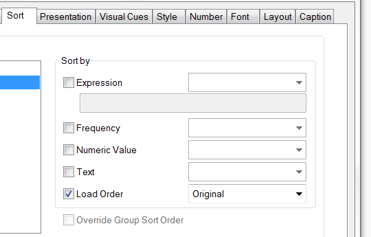
The Presentation pane of a Straight Table Chart provides an option to show or hide each individual column. The decision to Show/Hide may also be specified as a conditional. If the condition evaluates to true, the column will be displayed.

Hidden columns are calculated and are “present” as data in the chart. The resulting column  is not visible in the rendered chart. Let’s look at a use case for this feature.

Straight Tables expressions may reference other columns in the table as data items.

The Net Sales expression above uses column labels:

=[Gross Sales] – [Sales Tax] – Cost

We can hide the intermediate columns and still use them as data to calculate the “Net Sales” column. This is a useful technique for building up a complex calculation.

The final chart displays only the “Net Sales” column.

The same hidden column technique is available in Bar and Line Charts as well. However, in this case we hide the column by unchecking the Bar (or Line) Display Option  on the Expression pane.

Let’s turn our attention to hiding Dimensions. In the example below, if we want one row for each Order we must include a unique field like OrderId in the Dimensions.

What if we don’t want to display the OrderId, but still want one row per Order? If we remove OrderId from Dimensions the table rolls up to a row for each Description value. That is not what we want.

We can get the desired result by leaving OrderId in the Dimensions and hiding the column on the Presentation pane.

A hidden dimension column participates in defining the rows of a chart. This is a useful feature, although it’s utility is not always obvious.

Qlikview Version 11 introduced  the Dimension/Expression Conditional property. This is enabled by checking Conditional (on the Dimensions or Expressions pane) and supplying an expression to be evaluated. If the expression evaluates to True, the column will be calculated. If False, the column will not be calculated. If it is not calculated, it cannot be referenced by another expression.

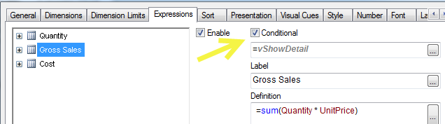
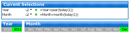
A common use for the Conditional property is to toggle columns on or off in a wide text chart.

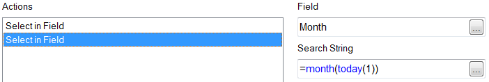
The button toggles the variable “vShowDetail” which is tested in the Expression conditional:

Another common use case is the “create your own chart” or “dynamic reporting” where users are allowed to pick Dimensions and Expressions from a list. This property — Dimension/Expression Conditional — is the correct way to implement this. If you instead implement the conditional in the Presentation pane, resources will be wasted calculating values that will not be displayed or referenced.

I find an interesting application for conditional Dimensions in Pivot Tables. I sometimes use buttons or other conditions to enable dimension levels. This presents the same output as Pivot table Expand/Collapse commands but without the clutter of the +/– buttons.

A QVW containing all the examples shown here may be downloaded from Qlikview Cookbook: Tutorial – About Column Visibility.

-Rob

A Customer showed me this stacked bar chart and asked how to “make the Goals a different color”. What he really wanted was to differentiate the Goal stacks from the Actual stacks — but still be able to associate the Channels (Consumer, Online,…).

Channel values are expected to change over time, so any hard-coding of Channel to color would require maintainence. Here’s the Background Color expression I suggested:

if(Type=’Goal’
,argb(96,255,255,255) bitand color(FieldIndex(‘Channel’,Channel))
,color(FieldIndex(‘Channel’,Channel))
) 

If that makes perfect sense to you, read no further. Otherwise let me break the expression down.

What we are doing in the expression is setting the Alpha value to “96” when “Type=Goal”. “Type=Actual” will retain the Alpha default of “255”.

Color codes in QV are made up of four numbers — Alpha, Red, Green, Blue — values which we can set in a color dialog or a color function. Alpha indicates the amount of transparency, ranging from 0 (fully transparent) to 255 (fully opaque). Colors functions without an explicit Alpha value like “RGB(0,128,0)” default to Alpha=255.

The function “Color(n)” returns the color code for the “Nth” position in the chart color palette.

FieldIndex(‘Field‘, Value) returns the position of  Value in Field (by load order).  This will generate a number for each distinct Channel value, regardless of how many Channel values are loaded. We are effectively assigning persistent colors because FieldIndex() is not affected by selections.

1. We use color(FieldIndex(‘Channel’,Channel)) to select color n from the palette.

2. If  Type=Goal  we use the boolean bitand operator to set the Alpha value for the selected color to “96” without modifying the RGB values. Adjust this 96 value for an effect of your liking.

-Rob

I’m always tickled to learn something new in QV, especially when it’s simple and elegant. swuehl, a prolific and respected contributor to QlikCommunity, answered this Community post with a brilliant solution.

The problem was how to calculate a Project (the Dimension) duration using dates from two different rows in the source table. I would have automatically reached for a script solution, Generic Load. But what if you don’t want to modify the script or don’t want the flattened model produced by Generic Load?

Swuehl’s solution computed the value in the chart using Set Analysis to fetch the needed values from the appropriate row.

only({<progress = {deployed}>} entry_date ) 
   – only({<progress = {started}>} entry_date)

The cleverness lies in using the only() aggregation function. Set Analysis can only be used in aggregation functions, so he used only() to enable specifying the Set.

I like it.

-Rob

My colleague Barry Harmsen on the QlikFix blog recently published some cool QV animations. Barry is the kid who’s math homework I copied because I was too busy playing volleyball.

Barry’s post referenced the work of Hans Rosling and gapminder.org. Hans Rosling is one of my data visualization heroes and I use Mr Rosling’s work as demonstration material when I teach Qlikview, particularly his widely viewed “Health and Wealth of Nations” time series animation.

Inevitably, after viewing “Health and Wealth of Nations” my students would ask “Can Qlikview do that?”. My answer used to be “I’m not sure”, but some time back I set out to recreate the same animation in QV. So the answer is now “yes”, but ironically, I haven’t had a student ask since I developed it. I have to wear an anticipatory grin and prompt the students with “Do you think Qlikvew can do that?”.

For the record, here’s the QV version of Gapminder’s “Health and Wealth of Nations”.  You can download a working QVW that includes the animation here. Click the green play button and watch it march through the years from 1800 to 2009.

I’m sometimes asked by developers “How do I make un-associated (gray) data disappear from listboxes?”. After some discussion as to why they want to do this, I usually attempt to convince them to not hide any data.

Gray data is an important part of the power of Qlikview — the associative experience.  Associative is the way our mind connects data. When I try to recall a face I may narrow my candidates by an attribute like hair color or where we met. But I don’t forget everyone else. I just take them out of focus.

I recall one of my first Qlikview “Wow!” moments when I saw the power of the associative process. I was working with a Industrial Safety analyst who was studying the effectiveness of various glove styles in preventing hand injuries. We had a database of injuries and a separate dataset of glove models in use by period and location.

Up to this point, the analyst had been working from static reports that counted injuries of interest by looking for “where BodyPart=’Hand'”.

We loaded the data into Qlikview. BodyPart  became a listbox. He selected “Hand” and the table charts displayed the same counts as the static reports. In the gray data we noticed a significant number of injuries for “Hend”, a misspelling of “Hand”. A simple click added those into the total. The analyst also discovered “finger” and “fingers” were of interest and added those. Furthermore, for certain glove styles — those with a gauntlet sleeve —  “forearm” should be added.

With just a few clicks the Analyst had greater accuracy in this important work. It was the display of gray data that allowed this to happen, along with the ability to quickly convert gray to green (selected).

So while there may be edge cases where it’s necessary to hide gray data, I generally find that displaying all data in the associative manner is a unique and special advantage of Qlikview.

I’ve posted in the past about setting “dynamic” (based on date) initial selections. The easiest method from the Developer perspective is to apply search expressions, save them in a bookmark, and apply the bookmark as an OnOpen action. The bookmark may also be selected by the user at any time to return to initial selections.


For example, to select the current year and month:


=Year=year(today(1))
=Month=month(today(1))


This selects the correct Year and Month. However, the current selections display is poor.  The search expression, rather than results, is displayed in the Current Selections box.

Alternatively, those same dynamic selections can be achieved via Actions assigned to the Document OnOpen Trigger. Using Actions will present a cleaner current selections view. Here are the two Actions we should assign to OnOpen to achieve the same selections — but with a better looking current selections display at the end.

The Current Selections Display will now be much more comprehensible to the user.

Can we provide a way for the user to return to the dynamic initial selections by utilizing a bookmark? Yes we can. Create a new bookmark, assign it an appropriate name (like “Current Period”) and note its ID (for example “BM02” — from the Bookmark, More menu). Add one more action to the OnOpen trigger.

The selection values will be calculated and the bookmark updated with the new values each time the document is opened. 


-Rob

I avoid using Caption Icons in sheet Objects. I prefer to teach users to right-click to access the same functionality. In V10, there is also the option to use a  “Menu” caption icon that provides the same options as right-click.

Here are my arguments for not using caption icons that duplicate the functionality available in right-click.

Note: I realize there are some limitations in the Ajax client prior to V9 that may require icons. My comments are directed at V9+.

1. The redundancy and visual clutter waste screen space and distract from the data. If you are a fan of Edward Tufte’s work, you’ll recognize this as “low Data-ink ratio” and “Chartjunk”.
2. They deemphasize icons that may be unique and important to a specific chart. These are things you want the user to notice, for example Help or Fast Change.
3. They force the designer to display a Caption even when a Caption is not desirable for the layout.
4. They keep users ignorant of the full power available, leading them to believe that they are limited to the functions offered by the displayed icons. Have you ever received a change request like “Please add the export to Excel function to chart X so we can export it.”?
5. Also on the ignorance theme, users don’t become aware of new functionality if you don’t add the new icons.